class: center, middle, inverse, title-slide .title[ # Importing/Exporting Data ] .subtitle[ ## <br><br> Introduction to Data Science ] .author[ ### University of Edinburgh ] .date[ ### <br> 2024/2025 ] --- class: middle # Reading and writing rectangular data --- ## Ways of rectangular data may be stored .pull-left[ - comma delimitation <img src="img/data_structures/delim_comma.png" width="100%" style="display: block; margin: auto;" /> - semicolon delimitation <img src="img/data_structures/delim_semicolon.png" width="100%" style="display: block; margin: auto;" /> ] .pull-right[ - tab delimitation <img src="img/data_structures/delim_tab.png" width="100%" style="display: block; margin: auto;" /> - MS Excel encoding <img src="img/data_structures/excel.png" width="100%" style="display: block; margin: auto;" /> ] --- ## Reading data .pull-left[ **readr** - part of tidyverse - `read_csv()` - comma delimited files - `read_csv2()` - semicolon separated files (common in countries where , is used as the decimal place) - `read_tsv()` - tab delimited files - `read_delim()` - reads in files with any delimiter - ... **readxl** - _not_ part of tidyverse - `read_excel()` - read xls or xlsx files - ... ] .pull-right[ <img src="img/readr.png" width="35%" style="display: block; margin: auto;" /> <br> <img src="img/readxl.png" width="35%" style="display: block; margin: auto;" /> ] --- ## Reading data (skipping first few lines) .pull-left[ ``` r library(readxl) tube <- read_excel( path = "data/tube-stations.xlsx") glimpse(tube) ``` ``` ## Rows: 10 ## Columns: 5 ## $ `Tube station data` <chr> "Some tube… ## $ ...2 <chr> NA, "Line"… ## $ ...3 <chr> NA, "Zone"… ## $ ...4 <chr> NA, "Opene… ## $ ...5 <chr> NA, "Numbe… ``` ] .pull-right[ ``` r tube <- read_excel( path = "data/tube-stations.xlsx", skip = 2) glimpse(tube) ``` ``` ## Rows: 8 ## Columns: 5 ## $ Station <chr> … ## $ Line <chr> … ## $ Zone <chr> … ## $ Opened <chr> … ## $ `Number of passengers (millions, 2019)` <chr> … ``` ] --- ## Writing data to file Most read functions have a corresponding write function. ``` r write_csv(tube, file = "data/tube-station-comma.csv") write_csv2(tube, file = "data/tube-station-semicolon.txt") write_tsv(tube, file = "data/tube-station-tab.txt") ``` Note, a file write is a quiet function (it does return anything to R!) ``` r glimpse( read_tsv("data/tube-station-tab.txt") ) ``` ``` ## Rows: 8 ## Columns: 5 ## $ Station <chr> "Russell Square", "Heathrow Te… ## $ Line <chr> "Piccadilly", "Piccadilly", "J… ## $ Zone <chr> "1", "6", "4", "3", "2", "6", … ## $ Opened <chr> "15 December 1906", "16 Decemb… ## $ `Number of passengers (millions, 2019)` <dbl> 12.270, 7.880, 4.550, 7.670, 4… ``` --- class: middle # Variable names --- ## Data with bad names ``` r edibnb_badnames <- read_csv("data/edibnb-badnames.csv") names(edibnb_badnames) ``` ``` ## [1] "ID" "Price" "neighbourhood" ## [4] "accommodates" "Number of bathrooms" "Number of Bedrooms" ## [7] "n beds" "Review Scores Rating" "Number of reviews" ## [10] "listing_url" ``` ... but R doesn't allow spaces in variable names ``` r ggplot(edibnb_badnames, aes(x = Number of bathrooms, y = Price)) + geom_point() ``` ``` ## Error: <text>:1:40: unexpected symbol ## 1: ggplot(edibnb_badnames, aes(x = Number of ## ^ ``` --- ## Option 1 - Manual edit - Edit the column names in the raw data file to `snake_name` style - OK, provided that you are only ever working with one file - Method is not _reproducible_ if developing a data flow where your data file may be updated - Can this be done in the code? --- ## Option 2 - Define column names ``` r edibnb_col_names <- read_csv("data/edibnb-badnames.csv", skip = 1, col_names = c("id", "price", "neighbourhood", "accommodates", "bathroom", "bedroom", "bed", "review_scores_rating", "n_reviews", "url")) ``` ``` ## Rows: 13245 Columns: 10 ## ── Column specification ──────────────────────────────────────────────────────── ## Delimiter: "," ## chr (2): neighbourhood, url ## dbl (8): id, price, accommodates, bathroom, bedroom, bed, review_scores_rati... ## ## ℹ Use `spec()` to retrieve the full column specification for this data. ## ℹ Specify the column types or set `show_col_types = FALSE` to quiet this message. ``` ``` r names(edibnb_col_names) ``` ``` ## [1] "id" "price" "neighbourhood" ## [4] "accommodates" "bathroom" "bedroom" ## [7] "bed" "review_scores_rating" "n_reviews" ## [10] "url" ``` --- ## Option 3 - `clean_names` to snake_case ``` r library(janitor) #may need to run: install.packages("janitor") ``` ``` r edibnb_clean_names <- read_csv("data/edibnb-badnames.csv") %>% clean_names() ``` ``` ## Rows: 13245 Columns: 10 ## ── Column specification ──────────────────────────────────────────────────────── ## Delimiter: "," ## chr (2): neighbourhood, listing_url ## dbl (8): ID, Price, accommodates, Number of bathrooms, Number of Bedrooms, n... ## ## ℹ Use `spec()` to retrieve the full column specification for this data. ## ℹ Specify the column types or set `show_col_types = FALSE` to quiet this message. ``` ``` r names(edibnb_clean_names) ``` ``` ## [1] "id" "price" "neighbourhood" ## [4] "accommodates" "number_of_bathrooms" "number_of_bedrooms" ## [7] "n_beds" "review_scores_rating" "number_of_reviews" ## [10] "listing_url" ``` --- class: middle # Variable types --- ## Which type is variable `x`? .pull-left[ <img src="img/df-na.png" width="100%" /> ] .pull-right[ ``` r read_csv("data/df-na.csv") ``` ``` ## Rows: 9 Columns: 3 ## ── Column specification ────────────────────────── ## Delimiter: "," ## chr (3): x, y, z ## ## ℹ Use `spec()` to retrieve the full column specification for this data. ## ℹ Specify the column types or set `show_col_types = FALSE` to quiet this message. ``` ``` ## # A tibble: 9 × 3 ## x y z ## <chr> <chr> <chr> ## 1 1 a hi ## 2 <NA> b hello ## 3 3 Not applicable 9999 ## 4 4 d ola ## 5 5 e hola ## 6 . f whatup ## 7 7 g wassup ## 8 8 h sup ## 9 9 i <NA> ``` ] --- ## Option 1. Explicit NAs ``` r read_csv("data/df-na.csv", na = c("", "NA", ".", "9999", "Not applicable")) ``` .pull-left[ <img src="img/df-na.png" width="100%" /> ] .pull-right[ ``` ## # A tibble: 9 × 3 ## x y z ## <dbl> <chr> <chr> ## 1 1 a hi ## 2 NA b hello ## 3 3 <NA> <NA> ## 4 4 d ola ## 5 5 e hola ## 6 NA f whatup ## 7 7 g wassup ## 8 8 h sup ## 9 9 i <NA> ``` ] --- ## Option 2. Specify column types ``` r read_csv("data/df-na.csv", col_types = list(col_double(), col_character(), col_character())) ``` ``` ## # A tibble: 9 × 3 ## x y z ## <dbl> <chr> <chr> ## 1 1 a hi ## 2 NA b hello ## 3 3 Not applicable 9999 ## 4 4 d ola ## 5 5 e hola ## 6 NA f whatup ## 7 7 g wassup ## 8 8 h sup ## 9 9 i <NA> ``` --- ## Column types .small[ **type function** | **data type** ------------------ | ------------- `col_character()` | character `col_date()` | date `col_datetime()` | POSIXct (date-time) `col_double()` | double (numeric) `col_factor()` | factor `col_guess()` | let readr guess (default) `col_integer()` | integer `col_logical()` | logical `col_number()` | numbers mixed with non-number characters `col_numeric()` | double or integer `col_skip()` | do not read `col_time()` | time ] --- class:middle # Case study: Favourite foods --- ## Favourite foods <img src="img/fav-food/fav-food.png" width="80%" style="display: block; margin: auto;" /> ``` r *fav_food <- read_excel("data/favourite-food.xlsx") fav_food ``` ``` ## # A tibble: 5 × 6 ## `Student ID` `Full Name` favourite.food mealPlan AGE SES ## <dbl> <chr> <chr> <chr> <chr> <chr> ## 1 1 Sunil Huffmann Strawberry yoghurt Lunch only 4 High ## 2 2 Barclay Lynn French fries Lunch only 5 Midd… ## 3 3 Jayendra Lyne N/A Breakfast and lu… 7 Low ## 4 4 Leon Rossini Anchovies Lunch only 99999 Midd… ## 5 5 Chidiegwu Dunkel Pizza Breakfast and lu… five High ``` --- ## Variable names <img src="img/fav-food/fav-food-names.png" width="80%" style="display: block; margin: auto;" /> ``` r fav_food <- read_excel("data/favourite-food.xlsx") %>% * clean_names() fav_food ``` ``` ## # A tibble: 5 × 6 ## student_id full_name favourite_food meal_plan age ses ## <dbl> <chr> <chr> <chr> <chr> <chr> ## 1 1 Sunil Huffmann Strawberry yoghurt Lunch only 4 High ## 2 2 Barclay Lynn French fries Lunch only 5 Midd… ## 3 3 Jayendra Lyne N/A Breakfast and lunch 7 Low ## 4 4 Leon Rossini Anchovies Lunch only 99999 Midd… ## 5 5 Chidiegwu Dunkel Pizza Breakfast and lunch five High ``` --- ## Handling NAs <img src="img/fav-food/fav-food-nas.png" width="80%" style="display: block; margin: auto;" /> ``` r fav_food <- read_excel("data/favourite-food.xlsx", * na = c("N/A", "99999")) %>% clean_names() fav_food ``` ``` ## # A tibble: 5 × 6 ## student_id full_name favourite_food meal_plan age ses ## <dbl> <chr> <chr> <chr> <chr> <chr> ## 1 1 Sunil Huffmann Strawberry yoghurt Lunch only 4 High ## 2 2 Barclay Lynn French fries Lunch only 5 Midd… ## 3 3 Jayendra Lyne <NA> Breakfast and lunch 7 Low ## 4 4 Leon Rossini Anchovies Lunch only <NA> Midd… ## 5 5 Chidiegwu Dunkel Pizza Breakfast and lunch five High ``` --- ## Make `age` numeric .pull-left-wide[ ``` r fav_food <- fav_food %>% * mutate( * age = if_else(age == "five", "5", age), * age = as.numeric(age) * ) glimpse(fav_food) ``` ``` ## Rows: 5 ## Columns: 6 ## $ student_id <dbl> 1, 2, 3, 4, 5 ## $ full_name <chr> "Sunil Huffmann", "Barclay Lynn", "… ## $ favourite_food <chr> "Strawberry yoghurt", "French fries… ## $ meal_plan <chr> "Lunch only", "Lunch only", "Breakf… ## $ age <dbl> 4, 5, 7, NA, 5 ## $ ses <chr> "High", "Middle", "Low", "Middle", … ``` ] .pull-right-narrow[ <img src="img/fav-food/fav-food-age.png" width="565" /> ] --- ## Socio-economic status .pull-left-wide[ ``` r fav_food %>% count(ses) ``` ``` ## # A tibble: 3 × 2 ## ses n ## <chr> <int> ## 1 High 2 ## 2 Low 1 ## 3 Middle 2 ``` ] .pull-right-narrow[ <img src="img/fav-food/fav-food-ses.png" width="75%" style="display: block; margin: auto;" /> ] .question[ Does the order of the `ses` categories make sense? ] --- ## Make `ses` factor .pull-left-wide[ ``` r fav_food <- fav_food %>% * mutate(ses = fct_relevel(ses, "Low", "Middle", "High")) fav_food %>% count(ses) ``` ``` ## # A tibble: 3 × 2 ## ses n ## <fct> <int> ## 1 Low 1 ## 2 Middle 2 ## 3 High 2 ``` ] --- ## Putting it altogether ``` r fav_food <- read_excel("data/favourite-food.xlsx", na = c("N/A", "99999")) %>% clean_names() %>% mutate( age = if_else(age == "five", "5", age), age = as.numeric(age), ses = fct_relevel(ses, "Low", "Middle", "High") ) fav_food ``` ``` ## # A tibble: 5 × 6 ## student_id full_name favourite_food meal_plan age ses ## <dbl> <chr> <chr> <chr> <dbl> <fct> ## 1 1 Sunil Huffmann Strawberry yoghurt Lunch only 4 High ## 2 2 Barclay Lynn French fries Lunch only 5 Midd… ## 3 3 Jayendra Lyne <NA> Breakfast and lunch 7 Low ## 4 4 Leon Rossini Anchovies Lunch only NA Midd… ## 5 5 Chidiegwu Dunkel Pizza Breakfast and lunch 5 High ``` --- ## Out and back in ``` r write_csv(fav_food, file = "data/fav-food-clean.csv") fav_food_clean <- read_csv("data/fav-food-clean.csv") ``` ``` r fav_food_clean %>% count(ses) ``` ``` ## # A tibble: 3 × 2 ## ses n ## <chr> <int> ## 1 High 2 ## 2 Low 1 ## 3 Middle 2 ``` .question[ What happened to the order of `ses` categories? ] --- ## `read_rds()` and `write_rds()` - CSVs can be unreliable for saving interim results if there is specific variable type information you want to hold on to. - An alternative is RDS files ('R data single'), you can read and write them with `read_rds()` and `write_rds()`, respectively. ``` r write_rds(fav_food, file = "data/fav-food-clean.rds") fav_food_clean <- read_rds("data/fav-food-clean.rds") fav_food_clean %>% count(ses) ``` ``` ## # A tibble: 3 × 2 ## ses n ## <fct> <int> ## 1 Low 1 ## 2 Middle 2 ## 3 High 2 ``` --- class: middle # Other types of data --- ## Other types of data importing - **googlesheets4:** Google Sheets - **haven**: SPSS, Stata, and SAS files - **DBI**, along with a database specific backend (e.g. RMySQL, RSQLite, RPostgreSQL etc): allows you to run SQL queries against a database and return a data frame - **jsonline**: JSON - **xml2**: xml - **rvest**: web scraping - **httr**: web APIs - **sparklyr**: data loaded into spark <br> ⬇️ You may need to install specialised R packages to read data from a specific format --- class: middle # Using RStudio GUI (Graphical User Interface) --- ## Importing CSV data - We've talked about the `read_csv` function - The options are a little bit fiddly, especially for wide datasets with many variables - You have to inspect the dataset manually to get it right ``` r tube <- read_csv("data/tube-stations.csv") ``` ``` ## Warning: One or more parsing issues, call `problems()` on your data frame for details, ## e.g.: ## dat <- vroom(...) ## problems(dat) ``` ``` ## Rows: 7 Columns: 2 ## ── Column specification ──────────────────────────────────────────────────────── ## Delimiter: "," ## chr (2): Station; Line; Zone; Opened; Number of passengers (millions, 2019) ## ## ℹ Use `spec()` to retrieve the full column specification for this data. ## ℹ Specify the column types or set `show_col_types = FALSE` to quiet this message. ``` Well, this doesn't seem to have worked! Let's look at the dataset… --- ## Tube stations data ``` r tube ``` ``` ## # A tibble: 7 × 2 ## `Station; Line; Zone; Opened; Number of passengers (millions` `2019)` ## <chr> <chr> ## 1 Russell Square; Piccadilly; 1; 15-DEC-1906; 12.27 <NA> ## 2 Heathrow Terminals 1 2, 3; Piccadill… ## 3 Kingsbury; Jubilee; 4; 10-DEC-1932; 4.55 <NA> ## 4 Tooting Bec; Northern; 3; 13-SEP-1926; 7.67 <NA> ## 5 Warwick Avenue; Bakerloo; 2; 31-JAN-1915; 4.00 <NA> ## 6 Upminster Bridge; District; 6; 17-DEC-1932; 1.11 <NA> ## 7 Battersea Power Station; Northern; 1; 1-JAN-3000; NA <NA> ``` - The separators are semicolons, not commas! - So we could use `read_csv2` - but we have to remember that! - Is there an easier way? --- class: inverse background-image: url("img/GUI/From-text-readr.png") ## The "Import Dataset" menu - **Environment** tab (top-right pane) - Several options! Choose **From Text (readr)...**. --- class: inverse background-image: url("img/GUI/Import-box.png") background-size: contain --- class: inverse background-image: url("img/GUI/Preview-1.png") background-size: contain --- class: inverse background-image: url("img/GUI/Preview-2.png") background-size: contain --- ## Choosing a data type from drop-down menu .pull-left[ For the "Zone" column .center[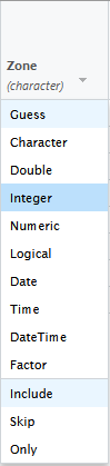] ] .pull-right[ For the "Opened" column .center[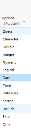] ] --- ## Date formats The default isn't right! Our dates are of the form `01-JAN-1900`, so we need to type `%d-%b-%Y` into the box. (`%b` encondes 3 character months, run `help(col_date)` for more on syntax) .pull-left[ .center[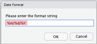] ] .pull-right[ .center[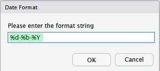] ] --- ## Importing from a CSV using the GUI .center[] - All the data types are correct - Note the non-integer Zone has become an `NA` … - … but not all NAs have been removed! --- ## Importing from a CSV using the GUI .center[] - We can run the code directly from the dialogue box, but that won't help with reproducibility/portability of the code - Instead, click the clipboard button (📋) to copy the code into yout editor. --- ## Importing from a CSV using the GUI ``` r #library(readr) tube_stations <- read_delim("data/tube-stations.csv", delim = ";", escape_double = FALSE, col_types = cols(Zone = col_integer(), Opened = col_date(format = "%d-%b-%Y")), trim_ws = TRUE) ``` ``` ## Warning: One or more parsing issues, call `problems()` on your data frame for details, ## e.g.: ## dat <- vroom(...) ## problems(dat) ``` It gives us the `readr` library, but if we've already imported the tidyverse we don't need to include that line, and can delete it. The warning message here is fine---it's telling us that "`not in a zone`" is not an integer, which we already know! --- ## Importing from a CSV using the GUI Let's prove it worked! ``` r tube_stations %>% summarise(mean_date = mean(Opened), med_zone = median(Zone, na.rm = T)) ``` ``` ## # A tibble: 1 × 2 ## mean_date med_zone ## <date> <int> ## 1 2056-05-13 3 ``` - The mean date is in the future because we haven't corrected that Year 3000 date yet! - .small[FYI, Battersea underground station opened in 20-SEP-2021.] --- ## Our data in an Excel file .center[] --- class: inverse background-image: url("img/GUIxl/From-text-readr.png") ## The "Import Dataset" menu - **Environment** tab (top-right pane) - Now we want **From Excel...**. --- class: inverse background-image: url("img/GUIxl/Import-box.png") background-size: contain --- class: inverse background-image: url("img/GUIxl/Preview-1.png") background-size: contain --- ## Importing from Excel using the GUI .center[] - We need to specify the range of cells in which the data are stored (or use the **Skip:** field) - The **Name:** field is the name under which we'll store the data once imported - Choose something different to avoid overwriting! --- ## Importing from Excel using the GUI .center[] - Check and edit the data types for each variable - We don't get separate **double** and **integer** options here: all we can choose is **numeric** (we can fix that later) --- ## Importing from Excel using the GUI .center[] - Again, let's copy this out using the clipboard icon… ``` r library(readxl) tube_stations_excel <- read_excel("data/tube-stations.xlsx", range = "A3:E11", col_types = c("text", "text", "numeric", "text", "numeric")) ``` - I've suppressed the warnings (`warning = F` in the code chunk label) because it gives lots, for every time it changes the data type in a cell